


Unified Star Schema - Part 2
The Bridge


Last week, I covered part 1 of the Unified Star Schema and, as I mentioned, it was a history of the what and how of Data Warehousing to date. It didn’t take us into new territory, which is intentional, as this is what the second part of the book does and what I will write about from here on out.
Unified Star Schema - Part 1

Last week, I wrote a post about a core part of the Unified Star Schema - the “Puppini” Bridge. As I mentioned, I feel like this approach is one that is different enough, and potentially valuable enough, that I really want to deep dive into it. It has the potential to solve a lot of problems that make self-serve analytics more difficult and narrower in s…
The first thing covered in part 2 of the book is a new concept which is the key component of the Unified Star Schema: the Bridge or as some call it, the “Puppini” Bridge.
The aim of the Unified Star Schema (USS) is to solve some of the problems encountered with Data Warehousing in the past: data silos, duplicate data marts, highly complex snowflake schemas that result in fan traps and chasm traps… and so on. The Bridge is central to its ability to do this.
Unlike the relational model and Kimball-type modeling, which is intuitive, the Bridge is somewhat counter-intuitive. However, once you have understood it thoroughly, it opens many new possibilities. I think it’s important to note that USS doesn’t look to replace the relational model, but to provide a useful abstraction that builds on top of it. Construction of the Bridge and its Stages is not possible without an existing relational model (even if this model is not explicit).
The Bridge is a tabular data object, which could be a database table, view or semantic layer object, constructed of Stages. Each Stage represents one entity or table in an existing relational data model. The Stage represents the connectivity of this object in the data model by storing its primary and foreign keys. The USS suggests a naming convention when constructing Stages, which I will follow, to ensure that keys are unique, consistent, easy to find and understand.
The Stage for one table is quite simple and may be as little as the name of the Stage and its primary key. The Bridge is a union of all of the Stages in the data model, meaning that Stages become quite sparse as they expand, to have null columns where other Stages have keys that they do not. Two Stages only have the same columns filled (excluding Stage name) when they have the same keys. In modern columnar data warehouses, this sparseness doesn’t usually result in inefficient data storage - tables are compressed well, with null or single value columns ranges taking up very little space.
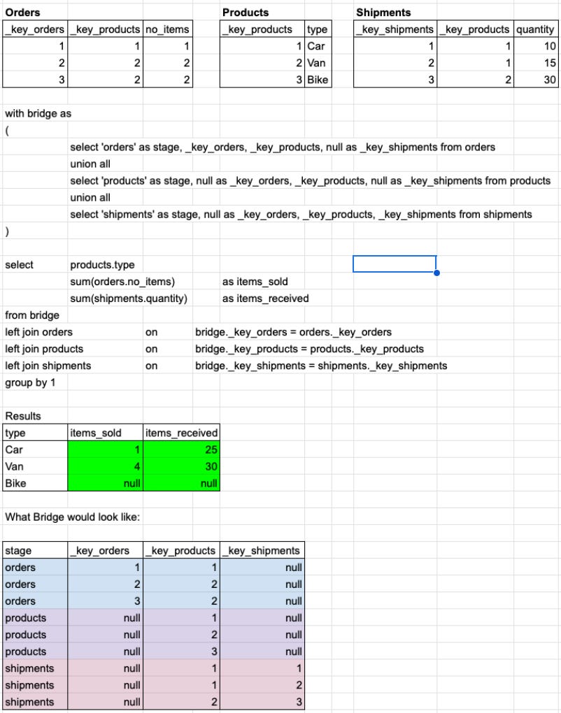
I’ve recreated the example data model I shared a couple of weeks ago, above, to illustrate the chasm trap. In the example, I make the Bridge using a CTE to show how to construct it, but, in reality, it could be created elsewhere beforehand.
There are tradeoffs as to how and when to create the Bridge. If you do it in the warehouse, it can end up large and costly/complex to partition and index. This could be mitigated by creating the stages individually and using a function to handle missing and misaligned columns to make union easier. In fact, if it was possible to filter the columns included in the union function to just those prefixed with _key_ or to an array of pre-defined keys, then you could use the original tables as the Stages, without needing to create more objects.
If the Bridge is created ephemerally each time, then it ends up being recreated very often. This can be made more efficient if the tool generating the code (BI or Semantic Layer, typically) injects filters into the ephemeral creation of the Bridge to ensure it only has the relevant keys to the timeframe or segment. Semantic layers typically have caches, and could offer the best of both worlds by caching ephemerally created Stages or Bridges for reuse in subsequent similar queries.
The issue of performance isn’t a blocker for using the USS, but is something where you will need to choose an appropriate configuration for your situation. There may be instances where you take different approaches in one company. An ephemeral Bridge approach for less-used and/or real-time datasets vs a materialised Bridge for daily updated gold datasets.
It would be much easier for a company if their semantic layer or BI tool handled the creation, maintenance, lazy-generation and/or caching of the Bridge for them.

As you can see, using the USS successfully avoids the chasm trap I illustrated a couple of weeks ago. It is not possible for rows in the Bridge to become duplicated, because it always joins many-to-one to the other tables’ primary keys. To calculate a measure, fields are brought in from other tables using these joins and then this extended Bridge is reduced to the granularity in the ‘group by’ statement.
There is a chapter dedicated to data loss in the book, and this example illustrates one example of avoided data loss. The query does output the Bike product type and the fact it has no sales or stock received from shipments. In typical queries, where joins filter the results, because there were no Bike sales or shipments, the join would filter out the Bike product from products. I think most SQL users have become accustomed to this, but it can be inconvenient and also misleading to those we present results to.
In the USS, the _key_products for Bike is always present in the Bridge and can’t be filtered out by any joins, which is why we don’t lose it. To query the relational model and get this result without the Bridge requires two earlier CTEs/subqueries/dbt models to sum and group products and shipments by _key_products and then left join these two to products, to achieve the same result:
with orders_by_product as
(
select _key_products, sum(no_items) items_sold
from orders
group by 1
),
shipments_by_product as
(
select _key_products, sum(quantity) items_received
from shipments
group by 1
)
select
products.type,
orders_by_product.items_sold,
shipments_by_product.items_received
from products
left join orders_by_product
on products._key_products = orders_by_product._key_products
left join shipments_by_product
on products._key_products = shipments_by_product._key_products
This kind of query, which does grouping in advance of joining the results together, is suboptimal. The groupings done early are specific to this query and not very reusable. It’s the sort of query I’ve written many times for adhoc analyses. It’s easy to get wrong and not great to read. Often, dashboards will run three separate queries to display the results that using the USS was able to show in one query above. Over time, fewer queries will generally result in lower data warehouse spend.
The Bridge query above, on the other hand, takes a similar form for any other query using it. The Bridge is readily reused by other queries of any grain. Bridge queries are aggregation queries - no aggregation has to be done beforehand. Generation of a query which aggregates to a user-specified grain is a core tenet of true self-serve analytics. There is no question of join direction when using the Bridge - it’s always the same. When writing the ad-hoc style query above to avoid the chasm trap, I ended up joining the dimension table to pre-aggregations of the two fact tables, which is the reverse of what ideally should happen.
I’ll go through more thoughts about the benefits of the USS next week.
The publisher of the Unified Star Schema, Technics Publications, have kindly shared a discount code “TP25” to purchase the book directly from their site. This way you get the book and the electronic PDF copy for less than just the book on Amazon!
London Analytics Meetup #7 is also scheduled for 17th September, which is the evening before Big Data London 2024. Francesco Puppini will be speaking - don’t miss out!
Sign up for the meetup here.